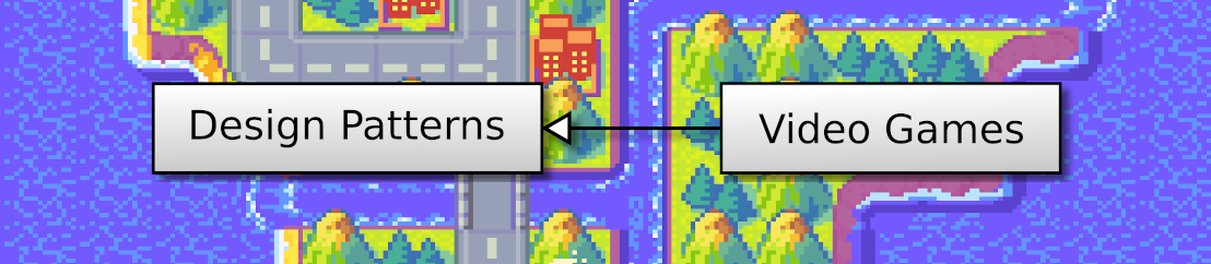
2D Strategy Game (16): Pathfinding
We move units using pathfinding, which computes the shortest path to reach a target cell.
This post is part of the 2D Strategy Game series
The player selects the knight with the left mouse button in the following video. Then, (s)he moves the mouse cursor, showing the shortest path to the pointed cell with the total movement cost. At last, (s)he moves the knight to a cell using the left mouse button:
Selection layer
The selection layer trick: we want to select a unit in the world with a left mouse click and add a selection box around:
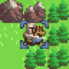
To get this result, we have to draw this selection box. A first approach directly renders the corresponding tile given the coordinates of the currently selected cell. This approach can look easier, but it requires computing the screen coordinates, which depend on many parameters.
A second approach uses the existing layer utilities to avoid another computation of the screen coordinates. Indeed, layer UI components render their tiles without the need to compute the coordinates explicitly. So, if we create a new SelectionLayer layer class, and a corresponding UI component SelectionComponent, then setting a cell in the selection layer will show a selection box.
In the WorldComponent class, which contains all layer components, we create these new objects:
self.__selectionLayer = SelectionLayer(world.size)
self.__selectionComponent = SelectionComponent(theme, state, self.__selectionLayer)
self.addComponent(self.__selectionComponent, cache=True)
Line 1 creates an instance of a new SelectionLayer class: it a child class of Layer, with some method related to selection. Note that we create it in WorldComponent in the ui package, not in the core package! It is related to UI, and the game logic does not need it. As a result, we can't add new values in the CellValue enum that lists world cell value types. Instead, we create a new SelectionValue enum with all cell value our selection layer can take: at the current moment, NONE (not selected) and SELECT (selected).
Lines 2-3 create and add an instance of a new SelectionComponent class, a child class of LayerComponent, that renders selection tiles. Then, we only need to set a selection layer cell to show a selection box. To this end, we add the following methods to the SelectionLayer class:
class SelectionLayer(Layer):
    def selectCell(self, cell: Tuple[int, int]):
        self.setValue(cell, SelectionValue.SELECT)
    def unselectCell(self, cell: Tuple[int, int]):
        self.setValue(cell, SelectionValue.NONE)
    ...
If we follow a call to one of these methods with a notification, then SelectionComponent will render the selection box, for instance:
selectionLayer.selectCell(cell)
selectionLayer.notifyCellChanged(cell)
Selection box tiles: we can render a selection box using a single tile, for instance:
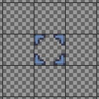
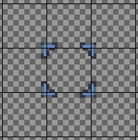
With a single tile, the selection box hides the unit a bit. To better surround the unit, we can use a larger tile, for instance, a 3x3 tile:
We render these tiles in the render() method of the SelectionComponent class:
def render(self, surface: Surface):
    ...
    valid = cells == SelectionValue.SELECT
    for dest, value, cell in renderer.coords(valid):
        rect = tilesRects[value][currentPlayerId]
        shift = vectorSubDiv2I(rect.size, tileSize)
        dest = vectorSubI(dest, shift)
        surface.blit(tileset, dest, rect)
We select the cell coordinates with a SelectionValue.SELECT value (line 3) and iterate through these coordinates (line 4). Then, for each cell, we select the tile corresponding to the current player (line 5). Since the selection tile is larger than a regular tile, we compute the shift that centers it on screen (line 6). The mathematical equivalent of this function package is: shift = (rect.size - normalTileSize) / 2. Finally, we apply the shift to the screen location (line 7) and blit the tile (line 8).
Distance map and pathfinding
Distance map: we compute the shortest between a selected cell and any other world cell using a Distance map. It is a 2D array with as many cells as there are world cells, where each cell contains the smallest cost to reach it:
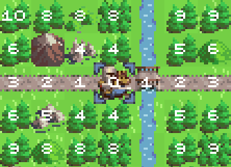
In this example, we selected the knight cell. On this cell, the move cost is zero. Then, the values around the selected cell are the costs for each direction. For instance, riding to the bridge on the right costs one point, and moving to a forest costs four points. This principle is repeated for each cell, except that we sum up all previous costs. For instance, going to the top-left cell costs 10 points: 1 (road) + 1 (road) + 4 (forest) + 4 (forest):
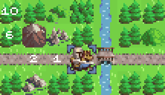
Since it is a distance map, the costs are always the lowest possible: if we try to reach the top-left cell from the right of the mountain, it costs 12 points: 4 (rocks) + 4 (forest) + 4 (forest).
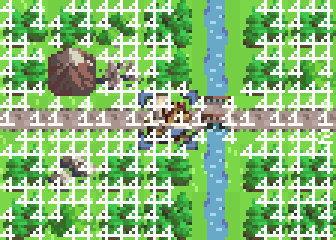
The distance map gives the data to compute the shortest path. The algorithm is simple: choose a target cell and always select a neighboring cell with the smallest value. Then, repeat until you reach a cell with zero cost. You can see more examples running the attached code: select the knight with the left mouse button, then hit F8 twice, showing the distance map.
Cost graph: computing the distance map requires a graph where nodes represent locations and edges the cost from one place to another. Here is an example with the knight node and its edges:
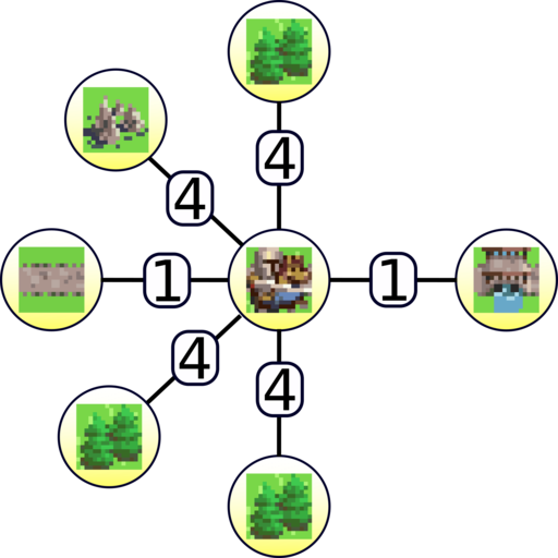
We value edges, where each value is the cost of moving from one node to another.
If you select the knight in the game and then hit F8 once, you can see the edge values:
This graph allows us to compute the distance map using the Dijkstra algorithm. However, before that, we must choose how we calculate the edge values.
Edge values: there is no unique way to compute these values, and we propose here one among others.
We first define costs for moving between cells of the same kind. We put these costs in a new MoveCost enum:
class MoveCost(IntEnum):
    ROAD_STONE = 1,
    ROAD_DIRT = 2,
    GROUND = 3,
    OBJECTS = 4,
    INFINITE = 10000
For instance, going from a ground cell to a ground cell costs 3 points. We also define an INFINITE cost representing cells that units can't walk on, like sea or mountain.
Then, we choose to define edge values as the maximum cost between two cells. For instance, moving from a stone road, a dirt road, or a ground cell to an object cell costs 4 points. It is a game design choice where we want to penalize leaving low-cost cells. For instance, if a unit is on a road tile, it costs a lot to hide in a forest. Other rules are possible; for instance, one could choose to compute the average cost between two cell costs.
Computation of the distance map: we create a new class DistanceMap, that handles the computation of a distance map in some world area.
We use the same trick as in the Layer class: we consider an area with extra rows/columns to handle borders. As a result, in the constructor of the DistanceMap class, we enlarge the area (lines 3-7):
def __init__(self, world: World, area: Tuple[int, int, int, int]):
    self.__world = world
    x1, y1, x2, y2 = area
    self.__area = (
        max(-1, x1 - 1), max(-1, y1 - 1),
        min(world.width + 1, x2 + 1), min(world.height + 1, y2 + 1)
    )
    self.__width = self.__area[2] - self.__area[0]
    self.__height = self.__area[3] - self.__area[1]
    self.__nodes = np.empty([self.__width, self.__height], dtype=np.int32)
    self.__edges = np.empty([self.__width, self.__height, 8], dtype=np.int32)
    self.__map = np.empty([self.__width, self.__height], dtype=np.int32)
We create Numpy arrays with this extended area (lines 10-12), knowing that we will only compute values for indices x from 1 to width-2 and y from 1 to height-2. Thanks to this trick, we won't have to check if we are outside the area when looking for neighbor cells. The nodes and edges arrays will contain the graph values and map the final distance map.
We compute the distance map in the compute() method of the DistanceMap class values. As much as possible, we use Numpy functions to get low computational time. We first fill all arrays with an infinite cost:
nodes.fill(MoveCost.INFINITE)
map.fill(MoveCost.INFINITE)
edges.fill(MoveCost.INFINITE)
Then, we start the computation of the cell costs in the node array. We assign to all ground cells in the area the corresponding move cost:
ground = world.ground.getArea(area)
selection = ground == CellValue.GROUND_EARTH
nodes[selection] = MoveCost.GROUND
We use the same approach to compute all cell costs in node (impassable, roads, objects, units). Then, we set border rows/columns to INFINITE:
nodes[:, 0] = MoveCost.INFINITE
nodes[:, -1] = MoveCost.INFINITE
nodes[0, :] = MoveCost.INFINITE
nodes[-1, :] = MoveCost.INFINITE
This step ensures that paths end when we reach the area's edges as if the world only contains the area.
The last step of cell costs computation assigns a zero cost at the location of the cell to reach (called source):
source = (source[0] - area[0], source[1] - area[1])
if source[0] < 0 or source[0] >= self.__width \
        or source[1] < 0 or source[1] >= self.__height:
    return
nodes[source] = 0
Note that we could set more cells with a zero cost, in which case the distance map would contain the shortest path to the closest source.
The graph edge values are the maximum cost between two cells in a given direction. We consider eight directions (from top-left to bottom-right) and thus compute eight values per cell in the edges array:
edges[1:, 1:, 0] = np.maximum(nodes[1:, 1:], nodes[:-1, :-1])
edges[1:, :, 1] = np.maximum(nodes[1:, :], nodes[:-1, :])
edges[1:, :-1, 2] = np.maximum(nodes[1:, :-1], nodes[:-1, 1:])
edges[:, 1:, 3] = np.maximum(nodes[:, 1:], nodes[:, :-1])
edges[:, :-1, 4] = np.maximum(nodes[:, :-1], nodes[:, 1:])
edges[:-1, 1:, 5] = np.maximum(nodes[:-1, 1:], nodes[1:, :-1])
edges[:-1, :, 6] = np.maximum(nodes[:-1, :], nodes[1:, :])
edges[:-1, :-1, 7] = np.maximum(nodes[:-1, :-1], nodes[1:, 1:])
This computation is fast and compact thanks to the rows/columns trick and the ability of Numpy to handle array slices. For instance, 1: means indices from 1 to the last, or :-1 from 0 to the penultimate.
The last step is the computation of the distance map using the Dijkstra algorithm:
queue = PriorityQueue()
map[source] = 0
queue.put((0, source))
while not queue.empty():
    _, cell = queue.get()
    x, y = cell
    costs = map[x, y] + edges[x, y]

    # Top Left
    cellTo = (x - 1, y - 1)
    cost = int(costs[0])
    if map[cellTo] > cost:
        map[cellTo] = cost
        queue.put((cost, cellTo))

    ...other directions...
This algorithm is, at the same time, simple and complex. It fits in a few lines but performs smart processing that leads to the distance map with linear complexity. Unfortunately, explaining this algorithm requires the introduction of graph theory, which is beyond the scope of this post: if you want to understand it, you can find many tutorials on the Internet.
Path computation: once we computed the distance map, we can get the shortest map to any cell of its area. We compute it in the getPath() method of the DistanceMap class:
def getPath(self, target: Tuple[int, int]) -> \
            Tuple[List[Tuple[int, int]], List[int]]:
    area, map = self.__area, self.__map
    target = (target[0] - area[0], target[1] - area[1])
    costs, path = [], []
    for i in range(100):
        cost = map[target]
        if cost == 0:
            break
        costs.append(cost)
        x, y = target
        path.append((x + area[0], y + area[1]))
        neighbors = np.delete(map[x - 1:x + 2, y - 1:y + 2].flatten(), 4)
        neighbors = neighbors[permutation]
        shift = index2shift[neighbors.argmin()]
        target = (x + shift[0], y + shift[1])
    return path, costs
We start by considering the cell we want to reach (in the target argument) and walk through the distance map until we find a cell with zero cost. At each step, we add the current target to the path, choose a neighboring cell with the smallest value, and set the target to this cell. If the distance map is valid, this process always succeeds. However, if for some reason it is not the case, the walk could last forever: it is the reason why we use a for loop with a fixed number of steps (line 6). If it happens, the resulting path is wrong, but the game does not freeze.
Lines 13-15 compute the shift from the current location x,y such as x+shift[0],y+shift[1] is a cell with the smallest value. To get this result, we first retrieve the neighboring values (line 13): map[x - 1:x + 2, y - 1:y + 2] extracts the 3x3 values around the current cell, flatten() turns this 2D array into a 1D array, and np.delete(...,4) removes the fourth item (it corresponds to the current cell).
The relative cell locations of costs are: top-left, left, bottom-left, top, bottom, top-right, right, and bottom-right. If there are equal neighboring values, we want to select non-diagonal directions. To get this behavior, we change the order with the following array (line 14):
permutation = np.array([1, 3, 4, 6, 0, 2, 5, 7])After line 14, the order is: left, top, bottom, right, top-left, bottom-left, top-right and bottom-right.
Finally, we use the following array to translate the index of the smallest value (line 15):
index2shift = [(-1, 0), (0, -1), (0, 1), (1, 0),
               (-1, -1), (-1, 1), (1, -1), (1, 1)]
This trick leads to a shorter and faster code than many if...elif... blocks.
Display cost numbers: we use the same trick as with the selection box. We consider a new range of 100 values in the selection layers, the first being SelectionValue.NUMBER_FIRST and the last SelectionValue.NUMBER_LAST. Then, we create as many corresponding tile numbers: SelectionValue.NUMBER_FIRST is tile "0", SelectionValue.NUMBER_FIRST+1 is tile "1", ..., SelectionValue.NUMBER_LAST-1 is tile "99". We also add a new showPath() method in the SelectionLayer class that sets all the cells of a given path:
def showPath(self, path: List[Tuple[int, int]], costs: List[int]):
    self.clearNumbers()
    for cell, cost in zip(path, costs):
        value = SelectionValue.NUMBER_FIRST + cost
        if value >= SelectionValue.NUMBER_LAST:
            continue
        self.setValue(cell, value)
Once we set path cells using this method, we trigger a content change notification, and SelectionComponent updates its rendering.
Move the unit
Play game mode: we create a new PlayGameMode class, child of DefaultGameMode, that handles most of the UI logic for selecting and moving a unit:
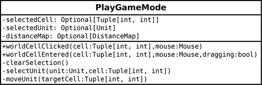
We capture the mouse click with the worldCellClicked() event of IComponentListener interface, as we did for editing the world. The WorldComponent class triggers it when the player clicks on a world cell and provides the world cell coordinates. Depending on the mouse button and current selection, we call selectUnit(), moveUnit() or clearSelection().
Select a unit: the selectUnit() method first updates the currently selected cell and unit (lines 2-3):
def __selectUnit(self, unit: Unit, cell: Tuple[int, int]):
    self.__selectedCell = cell
    self.__selectedUnit = unit
    self._selectionLayer.selectCell(cell)
    self._selectionLayer.notifyCellChanged(cell)

    x, y = cell
    radius = 31
    area = (x - radius, y - radius,
            x + radius + 1, y + radius + 1)
    self.__distanceMap = DistanceMap(self.world, area)
    self.__distanceMap.compute(cell)
Then, it sets a box in the selection layer (line 4). The selectCell() method of the SelectionLayer class assign a SelectionValue.SELECT to a cell of the selection layer. This assignment only changes the layer's content, as if it was game data, but does not necessarily lead to a visual update. As we did for other layer updates (in the game logic), we notify the cell change (line 5): the SelectionComponent class receives it and redraws itself.
The end of the method builds a distance map where the source cell is that of the selected unit. First, lines 7-10 compute a box area around the unit: the size of this area should be large enough to handle moves of the fastest units (right now, there is no limit to unit speed, so the value is arbitrary). Then, lines 11-12 create and compute the distance map.
Move a unit: the moveUnit() method creates a new MoveUnitCommand instance, schedules it, and clears the current selection:
def __moveUnit(self, targetCell: Tuple[int, int]):
    command = MoveUnitCommand(self.__selectedCell, targetCell)
    self._logic.addCommand(command)
    self.__clearSelection()
The MoveUnitCommand class moves a unit from one cell to another. It has the usual check() and execute() methods. The first one starts with many checks (not shown here) and computes the shortest path between the two cells:
def check(self, logic: Logic) -> bool:
    ...checks...
    fromX, fromY = self.__fromCell
    toX, toY = self.__toCell
    radius = 10
    area = (
        min(fromX, toX) - radius, min(fromY, toY) - radius,
        max(fromX, toX) + radius + 1, max(fromY, toY) + radius + 1
    )
    distanceMap = DistanceMap(world, area)
    distanceMap.compute(self.__fromCell)
    self.__path, costs = distanceMap.getPath(self.__toCell)
    return len(self.__path) != 0:
We first calculate an area that includes the path's beginning and end (lines 3-9). Note that we enlarge the area to handle the case of a detour. The shortest path computation is as we saw before; we store it in an attribute so we can use it in the execute() method (lines 10-12). Finally, we return True if the path is not empty (line 13).
The execute() method updates unit position and schedules another command if the path is not over:
def execute(self, logic: Logic):
    unitsLayer = logic.world.units
    unit = unitsLayer.getUnit(self.__fromCell)
    unitsLayer.setUnit(self.__fromCell, CellValue.NONE)
    targetCell = self.__path[-1]
    unitsLayer.setUnit(targetCell, CellValue.UNITS_UNIT, unit)
    unitsLayer.notifyCellChanged(self.__fromCell)
    unitsLayer.notifyCellChanged(targetCell)
    if len(self.__path) > 1:
        command = MoveUnitCommand(targetCell, self.__toCell)
        logic.addCommand(command)
We first retrieve the unit at the starting location (lines 1-2). Then, we remove it from this location (line 4), get the following position in the path (line 5), put the unit in this new location (line 6), and notify that the two cells have changed (lines 7-8). Finally, if the path is not over (line 9), we schedule a new move unit command starting from the current unit location (lines 10-11).
This implementation means that the unit moves one cell per game epoch. Furthermore, since we compute a distance at each command check, the unit can follow a different path than the initial one if other cells in the world change during its move. Note that it is a game design choice: we could also move it directly to the final position using a single command.
Final program
In the next post, we implement fighting mechanisms.